Given a spatial unit over the earth’s surface, which is variously known as catchment or watershed or basin, how incident rainfall becomes runoff at the catchment’s outlet — is probably the most fundamental question to a hydrologist. Hydrologic models (aka Rainfall Runoff Models) are the main tool that has been used by the hydrologists to answer this question quantitatively. A rainfall-runoff model is a simplification of a complex, non-linear, time and space varying hydrological process reality.

Over the years many types of hydrologic models have been developed and have been applied to various use cases. In a recently published work by Peters-Lidard et al. (2019), this development has been nicely captured and categorized into following six eras, as depicted in Figure 1.

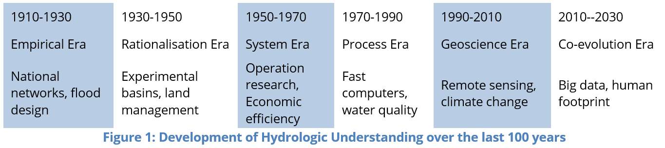
The development of the Hydrologic Modeling Center’s  Hydrologic Modeling System (HEC-HMS) started in the beginning of the Geoscience Era and it is still continuing in the current Co-evolution Era. The HEC-HMS is designed to simulate the precipitation-runoff process of dendritic watershed system. HEC-HMS is applicable for a range of spatial scales such as large river basin water supply and flood hydrology, and small urban or natural watershed runoff. For over last 30 years HEC-HMS has been used for various types of studies like water availability, urban drainage, flow forecasting, future urbanization impact, reservoir spillway design, flood damage reduction, floodplain regulation, and systems operation (see HEC-HMS’s online user manual).

HEC-HMS also has the capability of detailed representation of the sub-surface hydrologic processes and thereby also suitable for continuous simulation of rainfall-runoff process for the land cycle part of the hydrologic cycle. This article is intended as a concise primer on the continuous simulation of rainfall-runoff process for a general practitioner in the field of hydrology. The particular version on which this article is HEC-HMS 4.2.1.

The HEC-HMS Framework

Anatomy of HEC-HMS Projects

In HEC-HMS all modeling components are organized under a modular structure called “Project”. A project may consist of (up to) following six interdependent modules (sub-structures):

1. Basin Model: The physical watershed which is being modeled are represented in Basin Model by a combination of seven conceptual elements, 1) Sub-basin, 2) Reach, 3) Reservoir, 4) Junction, 5) Diversion, 6) Source and 7) Sink. To have a valid rainfall-runoff model, a basin model must contain at least one Sub-Basin Element. All other elements are optional and are to be included in Basin Model as per the requirement. Hydrologic computational algorithms (termed as “Methods” in HEC-HMS documentations) associated with these elements compute movement of water through the river basin being conceptualized within the Basin Model. The Basin Model requires inputs from “Control Specifications” module during the simulation run; it may also require fetching input data from “Time Series Data” and “Paired Data” modules depending on the “Methods” selected for its elements. A valid HEC-HMS project must contain at least one Basin Model.
2. Meteorologic Model: The Meteorologic Model of a Project calculates the (liquid) precipitation (PCP) and Potential Evapotranspiration (PET) required by the SBEs within the associated Basin Model. The Meteorologic Model can utilize both point and gridded PCP and has the capability to model frozen and liquid PCP through the snowmelt method. A Meteorologic Model always requires inputs from “Control Specifications”, “Time Series Data” modules; whereas its association with “Gridded Data” and “Paired Data” depends upon the “Methods” selected for meteorologic computations. A valid HEC-HMS project must contain at least one Meteorologic Model.
3. Time-Series Data: This module contains and manages all the time series data that are required by Meteorologic Model and Basin Model. All these time series are considered as point-source and thereby represented in this module as gauges, e.g., “Precipitation Gages”, “Evapotranspiration Gages” and “Discharge Gages” and so on.
4. Control Specifications: Control specifications are one of the main components in a project, even though they do not contain much parameter data. Their principal purpose is to control when simulations start and stop, and what time interval is used in the simulation. A valid HEC-HMS project must contain at least one “Control Specifications”.
5. Paired Data: Some of the hydrologic Methods/Models implemented in HEC-HMS require the use of paired data to describe inputs that are functional in form. Examples of paired data included user defined unit hydrograph for the Transform Method associated with an SBE, cross-section data associated with Routing Method of a Reach element and so on. “Paired Data” module contains and manages all such functional inputs required by the any/some methods selected in Basin Model or Meteorologic Model. Thus, presence of this module is optional and depending upon the Methods selected in Basin and/or Meteorologic Models, there may not be any “Paired Data” module in a Project
6. Gridded Data: Some of the Methods (like Gridded SCS Loss Method or Gridded SMA Loss Method) included in the program operates on a grid cell basis. This means that parameters must be entered for each grid cell. It also means that boundary conditions like PCP must be available for each grid cell. “Gridded Data” module contains and manages all such data.

Workflow of Procedures for a Typical SBE

Once a SBE has been set in the Basin Model, HEC-HMS GUI let the modeler associate it with five interconnected computational procedures. If we view these five interconnected set of procedures as a system, then PCP and PET at the sub-basin unit scale are the inputs to this system and discharge or flow (Q) at the sub-basin unit’s outlet is the output from the system. These five procedures are shown in Figure 2.

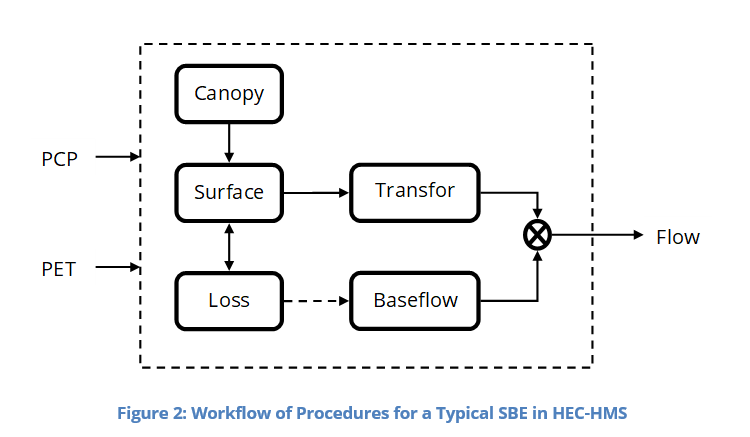
Each of these five procedures represents a component of hydrologic cycle as conceptualized in HEC-HMS. Arrows shown in Figure 2 indicate direction of the movement of water from one procedure to another. Note that dashed arrow connecting “Loss” and “Baseflow” procedures; this dashed arrow implies that output from the “Loss” procedure may or may not become input to the “Baseflow” procedure.

In each of these five procedures movement of water may be modeled using various Methods available within each procedure and selection of any particular Method is at the discretion of the modeler. Following list provides the inventory of methods associated with each procedure.

1. Canopy
   • Dynamic Canopy
   • Simple Canopy
   • Gridded Simple Canopy
2. Surface
   • Simple Surface
   • Gridded Simple Surface
3. Loss
   • Initial and Constant
   • Deficit and Constant
   • Exponential
   • Green and Ampt
   • Smith & Parlange
   • SCS Curve Number
   • Soil Moisture Accounting
   • Gridded Deficit and Constant
   • Gridded Green and Ampt
   • Gridded SCS Curve Number
   • Gridded Soil Moisture Accounting
4. Transform
   • Clark Unit Hydrograph
   • ModClark
   • SCS Unit Hydrograph
   • Snyder Unit Hydrograph
   • User-specified S-Graph
   • User-specified Unit Hydrograph
   • Kinematic Wave
5. Baseflow
   • Constant Monthly
   • Recession
   • Bounded Recession
   • Nonlinear Boussinesq
   • Linear Reservoir

It is not the purpose of this document to discuss technical details of each of these Methods. Rather some of these Methods shall be examined for more detailed enquiry after establishing a pathway for continuous simulation of rainfall-runoff processes and then each of those method shall be elaborated in detail. That is the task for the Part 2 of this article.

… to be continued.